Marek Kwiatkowski and Garry Gelade (1) (2) have included the visible angle of the goal (which is the angle at the shooter of the triangle shooter, left post, right post) in their xG-Models.
What I have not seen is a visualization of those angles and a discussion of how this concept can be further utilized beyond the use as an explanatory variable in xG models.
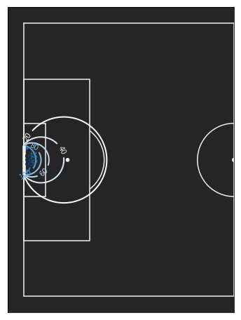
This is how open angles line up originating from the goal.
In shape it looks remarkably similar to how xG models ascribe goal probabilities.
As the angle increases with decreasing distance to the goal, understandingly the angle shows a high correlation with shot conversion.
Beyond using this angle as explanatory variable in xG Models, with Statsbomb Freeze Frame Data, we can also use this to start analyzing Goalkeeper Positioning and Defender Positioning.
So let’s look at an example.
import pandas as pd
import numpy as np
% matplotlib inline
import matplotlib.pyplot as plt
import matplotlib as mpl
import seaborn as sns
sns.set_style('darkgrid')
from math import pi
import math
from matplotlib.lines import Line2D
from FootiePy.drawpitch_ import drawpitch
fig, (ax1,ax2) = plt.subplots(2,1, figsize = (16,8))
ax1 = drawpitch(ax=ax1, measure = 'SB', orientation = 'vertical')
plt.sca(ax1)
plt.ylim(105,120.5)

x, y= 32, 116
plt.scatter(x, y, marker = 'x', label = 'Shooter');
plt.scatter(39, 119.5, marker = 'o', c = '#41ab5d', zorder = 999, label = 'Goalkeeper')

plt.plot([x, 36], [y, 120], '-', c = '#6baed6');
plt.plot([x, 44], [y, 120], '-', c = '#6baed6');
plt.plot([x, 40], [y, 120], '--', c = '#fc9272', label = 'Line To Center of Goal');
plt.legend(loc = (0.05, 0))

plt.sca(ax2)
ax2 = drawpitch(ax=ax2, measure = 'SB', orientation = 'vertical')
plt.ylim(105,120.5)

x, y= 32, 116
plt.scatter(x, y, marker = 'x', label = 'Shooter');
plt.scatter(38, 119.5, marker = 'o', c = '#41ab5d', zorder = 999, label = 'Goalkeeper')
line_l = plt.plot([x, 36], [y, 120], '-',c = '#6baed6');
line_r = plt.plot([x, 44], [y, 120], '-',c = '#6baed6');
line_c = plt.plot([x, 39], [y, 120], ls = '--', c = '#fc9272', label = 'rotated Line');
plt.legend(loc = (0.05, 0));
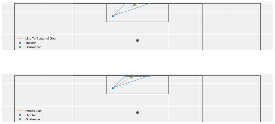
On the first plot it is easy to see that the angle at the near post (The triangle Shooter - GK - Near Post) is much bigger than the angle towards the far post.
Clearly, the line towards the goalcenter can not be the goalkeepers orientation point.
Rather, a better first orientation might be to position such that both angles towards near and far post are equally large.
We see (an approximation of) this on the second plot. This seems like a very reasonable position for the goalkeeper to take.
The reasoning behind this comes from game theory and is, that as the goalkeeper you should - without any further knowledge about the shooters tendencies - position such, that it is equally hard to score for him, regardless of him choosing to shoot at the near or far post. Otherwise a shooter could exploit your positioning by always shooting where you give him the higher expectation of scoring.
Now, it might still be that shots at the near post are scored more often if you took the above strategy of cutting both angles in half. It is fairly reasonable to assume that even from this positioning, a goalkeeper should tilt slightly towards the near post, as the distance towards the near post is closer.
To figure this out, one could try to look at a large dataset of shots and infer the optimal gk positioning from this.
From there you could also take into account shooter tendencies and if for example you are facing Arjen Robben just outside the box, maybe you could make it harder for him if you don’t deviate towards the near post as much as you usually do, as he is both much more likely to shoot at and convert shots at the far post (at least that’s what my eyes tell me).
So based on player specific tendencies, we might be able start looking for exploitive strategies and instruct our goalkeeper to position slightly differently.
Knowing what a solid or optimal positioning is in the first place is a requisite for this analysis.
fig, ax1 = plt.subplots(1,1, figsize = (16,4))
ax1 = drawpitch(ax=ax1, measure = 'SB', orientation = 'vertical')
plt.sca(ax1)
plt.ylim(105,120.5)

x, y = 41, 112
plt.scatter(x, y, marker = 'x', label = 'Shooter');
plt.scatter(38, 119.5, marker = 'o', c = '#41ab5d', zorder = 999, label = 'Goalkeeper')

line_l = plt.plot([x, 36], [y, 120], '-', c = '#6baed6');
line_r = plt.plot([x, 44], [y, 120], '-', c = '#6baed6');
line_c = plt.plot([x, 40.25], [y, 120], ls = '--', c = '#fc9272', label = 'rotated Line');
line_gk = plt.plot([x, 38], [y, 119.5], ls = '--', c = '#41ab5d', label = 'LineSGK');

plt.legend(loc = (0.05, 0));
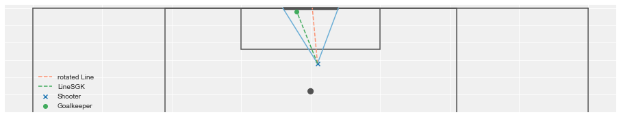
An application of this concept is also to look at the deviation of both angles.
Either the difference between them, or looking at the fraction the smaller angle has of the total angle.
In the above example, the goalkeeper is clearly cought out of position.
This will show in both approaches.
The advantage of using the absolute difference between both angles is that as you get closer to the goal, the open angle towards both posts increases (as seen on the first plot). Thus, seemingly small deviations from optimal positioning can actually mean a reasonably large angle difference.
This is what makes this a good variable for xG Models, as it reasonably captures an open goal.
The problem with this is though, that for shots from further out, the open angle becomes rather small, and thus you will only get smaller deviations.
To analyze positioning on those shots, it might be better to look at the relative deviation or the fraction.
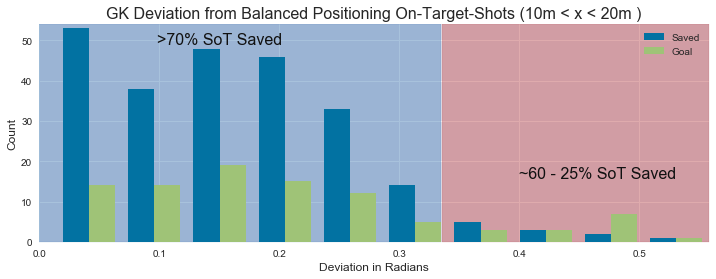
The next plot has to be taken with a huge grain of salt, because as I already mentioned, the angle increases as you get closer to the goal.
For this reason, the biggest angle deviations are all shots that are very close to the goal.
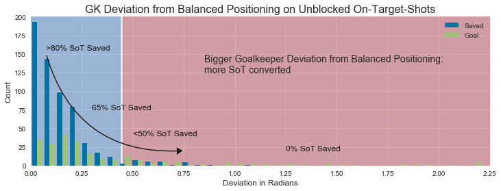
For shots from 10-20m distance, a small effect still shows. Again, this is very likely due to closer shots having a bigger open angle to the goal and thus being converted more often.
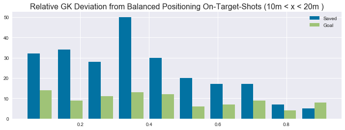
Looking at the relative deviation seems just a tiny bit more promising here.
Shots with a relative GK deviation of < 0.7 all show a goal probability of 0.7 - 0.8, bigger than that we see it decrease to around 65% and < 40% for shots in the biggest deviation bin.
Math: Computation of Angles
To figure out the angles, you can use the law of cosines.
It also generally helps to memorize ‘soh-cah-toa’
- Sine - Opposite over Hypotenuse, Cosine - Adjacent over Hypotenuse, Tangens - Opposite over Adjacent (shout out to Khan Academy) - whenever you are dealing with angles.